NMR Reporter Assays
NMR (Nuclear Magnetic Resonance) is not a high-throughput technique! However, it does have an extremely important role to play in the drug discovery process. In particular, NMR reporter assays can provide an efficient and reliable means of ranking compound binding over a wide range of affinities especially in the lower affinity range (μM to mM) where other biophysical techniques (such as SPR) may struggle to reliably quantify and rank binding. The quantitative information gleaned from NMR reporter assays can be used to guide medicinal chemistry efforts and develop an understanding of the structure activity relationship (SAR).
A reporter assay works by observing the displacement of a reporter molecule by a competitor molecule that binds to the same or overlapping site on a biomolecule. In the case of an NMR reporter assay the signal of the reporter is highly attenuated in the presence of the biomolecule of interest. Upon addition of a competitor molecule a recovery of the reporter signal intensity is observed. The percentage of displacement (recovery of signal) of the reporter can then be quantified and used to determine the affinity or \(IC_{50}\) of the competitor. This is a potentially efficient method of ranking compounds by affinity as it does not require large amounts of biomolecule (relative to 2D NMR methods) and it is possible to gain robust estimates of competitor affinities with as few as 3 data points per sample. Additionally, experimental times are much shorter as only 1D or pseudo 2D (2-3 \(T_2\) times) are required per dataset.
In general, three samples are required for an NMR reporter assay:
- Reporter only (negative control)
- Reporter + protein (positive control)
- Reporter + protein + competitor
It is also prudent to include an internal reference compound which does not interact with your biomolecule of interest. This internal control can be used to normalize your data and account for issues with sample homogeneity and shimming problems etc.
A good reporter molecule should have the following qualities:
- Specific stoichiometric (1:1) binder i.e. compound binding site is unique
- \(K_d\) known (this is not an absolute requirement but is necessary for quantification of \(K_i\) values)
- Large contrast in \(R_2\) between bound and free conditions in a concentration range that allows for acquisition of high signal to noise data.
- Fast \(k_{off}\) (fast exchange on NMR timescale). Should not have measurable kinetics by SPR (i.e. \(k_{off}\) > 2 \(s^{-1}\)).
A key advantage of NMR based reporter assays over other techniques such as fluorescence polarisation (FP) is that a sensitive assay can be achieved at much lower bound ligand fractions. For example, a typical FP assay requires an \(f_0\) of \(0.5-0.8\) whereas an NMR assay can be highly sensitive with \(f_0\) values as low as 0.003. This means that the measurable range of \(K_i\) values by NMR reporter assays is around 2 orders of magnitude wider (see IC50).
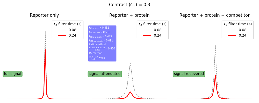
Below is a schematic showing the key experimental read-outs of a reporter assay (see Assay quality metrics for more details). On the left is the reporter only sample for which a sharp intense reporter signal is observed. Upon addition of protein to the sample the reporter signal is greatly attenuated (centre) due to the reporter binding to a specific site on the protein. Addition of a competitor molecule (right) leads to a recovery of signal intensity due competition for binding to the same site on the protein and hence a reduction in the bound fraction of reporter.
import nmrglue as ng
import numpy as np
import matplotlib
matplotlib.use('Agg')
import matplotlib.pyplot as plt

def I(I0: float, R2: float, tau: float) -> float:
   return I0*np.exp(-1.0*R2*tau)

def C2(R2_protein,R2_free):
   return (R2_protein - R2_free) / R2_protein

# setup parameters
R2_protein = 10.0 # s-1
R2_free = 2.0 # s-1
R2_comp = 5.0 # s-1
tau_long = 0.240 # s
tau_short = 0.080 # s
I0 = 1.0

I_free_short = I(I0,R2_free,tau_short)
I_free_long = I(I0,R2_free,tau_long)
I_protein_short = I(I0,R2_protein,tau_short)
I_protein_long = I(I0,R2_protein,tau_long)
I_comp_short = I(I0,R2_comp,tau_short)
I_comp_long = I(I0,R2_comp,tau_long)

peak_tau_short_free = ng.linesh.sim_NDregion((50,),['l'],[[(25,R2_free/np.pi)]],[I_free_short])
peak_tau_long_free = ng.linesh.sim_NDregion((50,),['l'],[[(25,R2_free/np.pi)]],[I_free_long])
peak_tau_short_protein = ng.linesh.sim_NDregion((50,),['l'],[[(25,R2_protein/np.pi)]],[I_protein_short])
peak_tau_long_protein = ng.linesh.sim_NDregion((50,),['l'],[[(25,R2_protein/np.pi)]],[I_protein_long])
peak_tau_short_comp = ng.linesh.sim_NDregion((50,),['l'],[[(25,R2_comp/np.pi)]],[I_comp_short])
peak_tau_long_comp = ng.linesh.sim_NDregion((50,),['l'],[[(25,R2_comp/np.pi)]],[I_comp_long])

contrast_R2 = C2(R2_protein,R2_free)
contrast_R2_text = r"$\frac{%.1f-%.1f}{%.1f}={%.1f}$"%(R2_protein,R2_free,R2_protein,contrast_R2)
ratio_protein = np.log(I_protein_long / I_protein_short)
ratio_free = np.log(I_free_long / I_free_short)
contrast_ratio = C2(ratio_protein,ratio_free)

contrast_ratio_text = r"$I_{80ms,free}=%.3f$"%(I_free_short) + "\n"
contrast_ratio_text += r"$I_{240ms,free}=%.3f$"%(I_free_long) + "\n"
contrast_ratio_text += r"$I_{80ms,protein}=%.3f$"%(I_protein_short) + "\n"
contrast_ratio_text += r"$I_{240ms,protein}=%.3f$"%(I_protein_long) + "\n"
contrast_ratio_text += "Ratio method\n"
contrast_ratio_text += r"$\frac{%.3f-%.3f}{%.3f}={%.3f}$"%(ratio_protein,ratio_free,ratio_protein,contrast_ratio)
contrast_ratio_text += "\n"+r"$R_2$ method"+"\n"
contrast_ratio_text += contrast_R2_text
bbox = dict(boxstyle="round",
            ec="g",
            fc="g",
            alpha=0.5)
bbox_caption = dict(boxstyle="round",
            ec="b",
            fc="b",
            alpha=0.5)

# make plot
fig, (ax1,ax2,ax3) = plt.subplots(1,3, figsize=(10,4))
long_dict = dict(linestyle="-",color="r",alpha=1.0,linewidth=2)
short_dict = dict(linestyle="--",color="k",alpha=0.5,linewidth=1)
ax1.plot(peak_tau_short_free,label=f"{tau_short}",**short_dict)
ax1.plot(peak_tau_long_free,label=f"{tau_long}",**long_dict)
ax2.plot(peak_tau_short_protein,label=f"{tau_short}", **short_dict)
ax2.plot(peak_tau_long_protein,label=f"{tau_long}", **long_dict)
ax3.plot(peak_tau_short_comp,label=f"{tau_short}", **short_dict)
ax3.plot(peak_tau_long_comp,label=f"{tau_long}", **long_dict)
ax1.text(0.0,0.3,"full signal",transform=ax1.transAxes, bbox=bbox)
ax2.text(0.0,0.3,"signal attenuated",transform=ax2.transAxes, bbox=bbox)
ax3.text(0.0,0.3,"signal recovered",transform=ax3.transAxes, bbox=bbox)
ax2.text(0.0,0.5,contrast_ratio_text,
         transform=ax2.transAxes,
         bbox=bbox_caption, color="white", fontsize="x-small")
for ax in [ax1,ax2,ax3]:
    ax.set_ylim(0,1)
    ax.legend(title=r"$T_2$ filter time (s)")
    ax.axis("off")
ax1.set_title("Reporter only")
ax2.set_title("Reporter + protein")
ax3.set_title("Reporter + protein + competitor")
plt.suptitle(r"Contrast $(C_2)$ = "+f"{contrast_R2:.1f}")
fname = "../static/contrast.png"
plt.tight_layout()
plt.savefig(fname)
return fname
Theory
Simple binding model
In the absence of a competitor the fraction of bound reporter is calculated using the following logic.
\begin{equation} K_d=\frac{[P][L]}{[PL]} \end{equation}Where \([P]\) and \([L]\) are the free protein and reporter concentrations and \([PL]\) is the bound concentration.
Using the mass conservation law, the free reporter and protein concentrations can be expressed in terms of the bound concentration and the total reporter and protein concentrations (\([L]_T\) and \([P]_T\), respectively):
\begin{equation} [P] = [P]_T - [PL] \end{equation} \begin{equation} [L] = [L]_T - [PL] \end{equation}Substituting these into the \(K_d\) equation gives
\begin{equation} K_d=\frac{([P]_T - [PL])([L]_T - [PL])}{[PL]} \end{equation}Which can be rearranged into a quadratic form to solve for \([PL]\).
\begin{equation} [PL] = \frac{([P]_T+[L]_T+K_d)-\sqrt{-([P]_T+[L]_T+K_d)^2 - 4[P]_T[L]_T}}{2} \end{equation}Since the fraction of bound reporter, \(f_0=\frac{[PL]}{[L_T]}\)
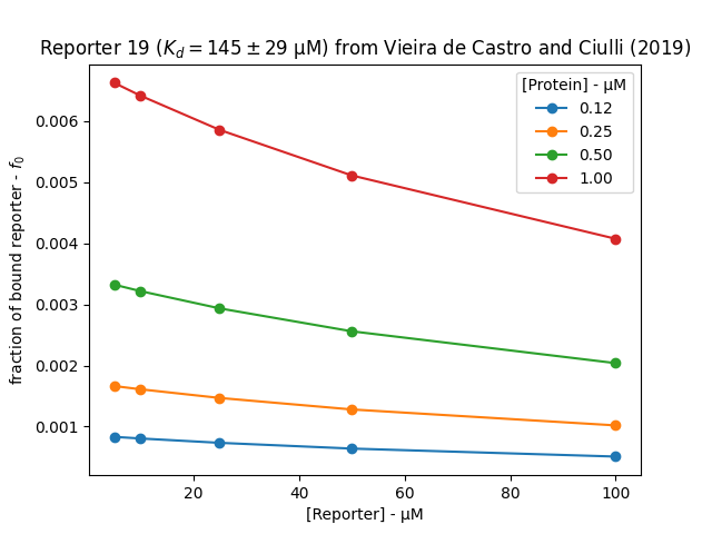
\begin{equation} f_0 = \frac{([P]_T+[L]_T+K_d)-\sqrt{-([P]_T+[L]_T+K_d)^2 - 4[P]_T[L]_T}}{2[L]_T} \end{equation}The plot below shows the bound fraction of reporter across a typical range of conditions that was tested by Vieira de Castro and Ciulli (2019). It is clear the protein concentration has a more significant effect on the bound fraction than the reporter concentration in this experimental range. Selecting a reporter and protein concentration becomes a trade off between having high \(C_2\), \(Z'\) and signal to noise. In this case, a good assay could be developed by selecting 50 μM reporter and 0.5-1 μM protein.
import numpy as np
import pandas as pd
import matplotlib.pyplot as plt
import matplotlib
matplotlib.use('Agg')

def f0(Pt: float, Lt: float, Kd: float) -> float:
    """ calculate fraction of bound ligand for 1:1 binding model

        Parameters
        ----------
        Pt : float
            total concentration of protein (M)
        Lt : float
            total concentration of ligand (M)
        Kd : float
            dissociation constant (M)

        Returns
        -------
        f : float
            fraction of ligand bound to protein

    """
    a = 1.0
    b = -1.0*(Pt+Lt+Kd)
    c = Pt*Lt
    return (-b-np.sqrt(b**2-4*a*c))/(2*Lt)

Pt = [0.125,0.250,0.500,1.000]
Lt = [5,10,25,50,100]
Kd = 145.0
fs = [["Protein","Reporter","Fraction"],]
for p in Pt:
    for l in Lt:
        f = f0(p,l,Kd)
        fs.append([p,l,f])
df = pd.DataFrame(fs[1:],columns=fs[0])
for name, group in df.groupby("Protein"):
    plt.plot(group.Reporter, group.Fraction,"o-",label=f"{name:.2f}")

plt.legend(title="[Protein] - μM")
plt.xlabel("[Reporter] - μM")
plt.ylabel(r"fraction of bound reporter - $f_0$")
plt.title("Reporter 19 ($K_d=145\pm29$ μM) from Vieira de Castro and Ciulli (2019)")
fname = "../static/fraction_bound.png"
plt.savefig(fname)
return fname
IC50
This is defined as the total competitor concentration (i.e. \([I]+[PI]\) or free competitor + bound competitor, resp) required to reduce the fraction of bound reporter ligand by 50% (\(f=f_0/2\)).
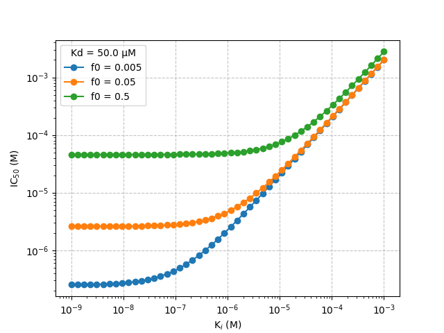
\begin{equation} IC_{50} = [I] + [PI] = \left( \frac{f_0 K_d}{(1-f_0)(2-f_0)} + \frac{f_0 L_0}{2} \right) \left( \frac{K_i(2-f_0)}{K_d f_0}+1 \right) \end{equation}The following graph demonstrates the range of \(IC_{50}\) values that it would be possible to measure using a competition assay for a given reporter \(K_d\) and fraction of bound receptor (\(f_0\)). The point at which the slope starts to tend towards 0 represents the lower limit of \(K_i\) that could be accurately measured by the assay. The smaller the \(f_0\) the greater the range of \(IC_{50}\) values that can be measured. NMR based reporter assays have the advantage of being sensitive to a wide range of \(IC_{50}\) values since these assays can be effectively performed at very low \(f_0\) values (\(f_0\) ~ 0.005). There is a trade off between achieving a low \(f_0\) and a high enough signal to noise (\(S/N\)) ratio and \(C_2\) value to give a robust assay.
from typing import Union
import numpy as np
import matplotlib
matplotlib.use('Agg')
import matplotlib.pyplot as plt

def calcIC50(Ki: Union[float, np.array], Kd: float,f0: float, L0: float) -> Union[float, np.array]:
    """ calculate IC50 value

        Parameters
        ----------
        Ki : float | np.array
            dissociation constant of competitor (M)
        Kd : float
            dissociation constant of reporter (M)
        f0 : float
            initial bound fraction of reporter
        L0 : float
            reporter concentration in (M)

        Returns
        -------
        ic50 : float | np.array
            concentration of competitor at which 50% displacement is achieved
            i.e. f = f0/2

    """
    ic50 = ((f0*Kd)/((1.0-f0)*(2.0-f0)) + (f0*L0)/2.0) * ((Ki*(2.0-f0))/(Kd*f0)+1.0)
    return ic50

Kd = 50e-6 # 50 μM
Ki = np.logspace(-9,-3)
L0 = 50e-6 # reporter concentration
f0s = [0.005,0.05,0.5] # fraction of bound ligand
for f0 in f0s:
    ic50 = calcIC50(Ki,Kd,f0,L0)
    plt.loglog(Ki,ic50,"o-",label=f"f0 = {f0}")
plt.grid(linestyle="--",alpha=0.75)
plt.ylabel("IC$_{50}$ (M)")
plt.xlabel("K$_{i}$ (M)")
plt.legend(title=f"Kd = {Kd*1e6:.1f} μM")
fname = "../static/ic50.png"
plt.savefig(fname)
return fname
Competitive binding model
An exact mathematical expression for competitive binding was defined by Wang (1994). For a simple 1:1 binding systems this involves solving a quadratic expression (see Simple binding model). However, for a competitive binding system a cubic expression must be solved (see https://en.wikipedia.org/wiki/Cubic_equation).
The following reaction scheme describes a competition experiment:
\begin{equation} [PL] + [I] \rightleftharpoons^{K_d} [P] + [L] + [I] \rightleftharpoons^{K_i} [PI] + [L] \end{equation}Where \([P]\), \([L]\) and \([I]\) are protein, reporter and competitor concentrations and \([PL]\) and \([PI]\) are the bound reporter and bound competitor concentrations respectively.
\begin{equation} K_d = \frac{[E][L]}{[EL]} \end{equation} \begin{equation} K_i = \frac{[E][I]}{[EI]} \end{equation}and
\begin{equation} L_0 = [L] + [EL] \end{equation} \begin{equation} I_0 = [I] + [EI] \end{equation} \begin{equation} E_0 = [E] + [EL] + [EI] \end{equation}The solution is found with a cubic expression and Wang (1995) showed that this can be solved using one of the unique and physically meaningful cubic roots shown below.
\begin{equation} a = K_d + K_i + L_0 + I_0 - E_0 \end{equation} \begin{equation} b = K_d(I_0-E_0) + K_i(L_0-E_0) + K_dK_i \end{equation} \begin{equation} \theta = \arccos \frac{-2a^3 + 9ab -27c}{2\sqrt{(a^2-3b)^3}} \end{equation} \begin{equation} d = 2\sqrt{(a^2-3b)}\cos{\frac{\theta}{3}}-a \end{equation} \begin{equation} [EL] = \frac{L_0d}{3K_dd} \end{equation}Since fraction of bound ligand is \(f=\frac{[EL]}{L_0}\) then
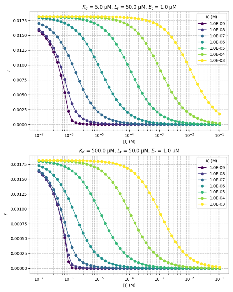
\begin{equation} f = \frac{d}{3K_d+d} \end{equation}Below is a plot showing simulated IC50 curves and demonstrates the range of \(Ki\) values that it would be possible to accurately measure using a model reporter system with the following experimental parameters:
| Parameter | Value |
|---|---|
| [Protein] | 1 μM |
| [Reporter] | 50 μM |
| Reporter \(K_d\) | 5 or 500 μM |
| \(K_i\) range | 1nM - 1mM |
Weaker reporters allow for a wider range of \(K_i\) measurements. Due to limitations with small molecule solubility it is unlikely that competitor concentrations greater than 1 mM are accessible. For example, this means that for a 5 μM \(K_d\) reporter the upper limit for observing full displacement is around the low μM \(K_i\) range, whereas for a weaker 500 μM \(K_d\) reporter almost 100% displacement can be achieved in the high μM \(K_i\) range upon addition of 1 mM of competitor.
from typing import Union
from cycler import cycler
import numpy as np
import matplotlib
from matplotlib import cm
matplotlib.use('Agg')
import matplotlib.pyplot as plt

def calcF(I: Union[float,np.array], Lt: float, Ki: float, Kd: float, Et: float) -> Union[float, np.array]:
    """ Calculate the fraction of bound reporter

        Wang (1995) defined an exact analytical solution to competitive binding.
        The following is a slight rearrangement of equation 14 to obtain the bound
        fraction of ligand based on the unique physically meaningful root of the
        cubic expression.

        Parameters
        ----------
        I : float | np.array
            concentration of competitor in M
        Lt : float
            total concentration of reporter `L_t` in M
        Ki : float
            `K_i` for the competitor in M
        Kd : float
            `K_d` for the reporter in M
        Et : float
            total concentration of protein `E_t` in M

        Returns
        -------
        f : float | np.array
            fraction of reporter bound to protein in the presence of competitor

    """
    a = Kd + Ki + Lt + I + Et
    b = (I-Et)*Kd + (Lt-Et)*Ki + Kd*Ki
    c = -Kd*Ki*Et
    theta = np.arccos((-2*a**3 + 9*a*b - 27*c)/(2*np.sqrt((a**2-3*b)**3)))
    d = 2*np.sqrt((a**2-3*b))*np.cos(theta/3) - a
    f = d / (3*Kd + d)
    return f

# some fancy colors
cmap = cm.viridis
len_cycle = 7
c = np.linspace(0,1,len_cycle)
custom_cycler = (cycler(color=[cmap(i) for i in c]))# +
                 #cycler(lw=np.arange(len_cycle)+1))

# configure plot
fig = plt.figure(figsize=(8,10))
ax1 = fig.add_subplot(211)
ax2 = fig.add_subplot(212)
ax1.set_prop_cycle(custom_cycler)
ax2.set_prop_cycle(custom_cycler)

# set parameters
Kis = np.logspace(-9,-3,len_cycle)
Lt = 50e-6
Kds = [5e-6,500e-6]
Et = 1e-6
I = np.logspace(-7,-1) # reporter concentration

# calculate and plot
axes = [ax1,ax2]
for Kd,ax in zip(Kds,axes):
    for Ki in Kis:
        Fw = calcF(I,Lt,Ki,Kd,Et)
        ax.semilogx(I,Fw,"o-",label=f"{Ki:.1E}")

    ax.grid(which='both',linestyle="--",alpha=0.75)
    ax.set_ylabel("$f$")
    ax.set_xlabel("[I] (M)")
    ax.set_title(r"$K_d$"+f" = {Kd*1e6:.1f} μM"+r", $L_t$"+ f" = {Lt*1e6:.1f} μM, " + r"$E_t$ " + f"= {Et*1e6:.1f} μM")
    ax.legend(title=r"$K_i$ (M)")
plt.tight_layout()
fname = "../static/fraction_bound_2.png"
plt.savefig(fname)
return fname
Assay quality metrics
Viriera and Ciulli (2019) have described an assay quality metric, \(C_2\), or contrast which is the fractional decrease in signal intensity in the presence of protein. Larger \(C_2\) values are usually preferred as this improves the dynamic range of the assay.
\begin{equation} C_2 = \frac{R_{2,+protein} - R_{2,free}}{R_{2,+protein}} \end{equation}Written in terms of intensity ratios this is equivalent to:
\begin{equation} C_2 = \frac{ ln \left[ \frac{ I_{\tau,long,+protein} }{ I_{\tau,short,+protein} }\right] - ln \left[ \frac{ I_{\tau,long,free} }{ I_{\tau,short,free} } \right]} {ln \left[\frac{I_{\tau,long,+protein}}{I_{\tau,short,+protein}}\right]} \end{equation}Where \(\frac{ I_{\tau,long,+protein} }{ I_{\tau,short,+protein}}\) is the ratio of reporter signal intensities at the long and short delay time \(\tau\) in the presence of protein and \(\frac{ I_{\tau,long,free} }{ I_{\tau,short,free}}\) is the ratio of reporter signal intensities in the absence of protein at the long and short delay times, respectively.
Another useful metric for defining the quality of the reporter assay is the \(Z'\) score which was first described by Zhang, Chung and Oldenburg (1999) for use in high-throughput screening (HTS) applications.
\begin{equation} Z' = 1-\frac{(3\sigma_{c+} + 3\sigma_{c-})}{|\mu_{c+}-\mu_{c-}|} \end{equation}Where \(\mu_{c+}\) and \(\mu_{c-}\) are the mean value for the positive (with protein) and negative (without protein) controls, respectively, and \(\sigma_{c+}\) and \(\sigma_{c-}\) are the standard deviations of the values for the positive and negative controls respectively. Calculation of a reasonable \(Z'\) score would require that one includes \(>3\) control samples ( ideally more!). \(Z'\) values of greater than 0.5 are considered to be good. However, as reported by Almeida, Panova and Walser (2021) \(Z'\) values greater than 0.8 should be achievable using the ratio of ratios method (see above) for an NMR reporter assay.
Practice
\(^1H\) vs \(^{19}F\)
The fluorine nucleus has advantages over proton for use as a reporter
- Background free
- Highly sensitive to weak binding due to high chemical shift anisotropy (CSA) and large chemical shift difference between free and bound states
This means that high \(C_2\) can be achieved relative to \(^1H\) at a given concentration leading to wider assay dynamic range.
Conditions
A good starting point is 1 μM protein and 50 μM reporter. However, there is no substitute for testing a few different protein and reporter concentrations to judge which provides the highest \(C_2\), \(Z'\) and \(\frac{S}{N}\) ratios. Vieira de Castro and Ciulli (2019) demonstrated this very clearly. It is also a good idea to test multiple reporters across a range of affinities. As was shown by Vieira de Castro and Ciulli (2019) the optimal reporter affinity can vary from 10s to 100s of μM.
NMR experiments
- T2 filtered experiments
- CPMG for \(^{19}F\)
- \(T_{1\rho}\) for \(^1H\)
References
- Spy vs. spy: selecting the best reporter for 19 F NMR competition experiments; Guilherme Vieira de Castro and Alessio Ciulli
- A Simple Statistical Parameter for Use in Evaluation and Validation of High Throughput Screening Assays; JH Zhang, TD Chung, KR Oldenburg
- NMR Reporter Assays for the Quantification of Weak-Affinity Receptor-Ligand Interactions; Teresa B Almeida, Stanislava Panova, Reto Walser
- Fluorescence polarization competition assay: the range of resolvable inhibitor potency is limited by the affinity of the fluorescent ligand;Xinyi Huang
- An exact mathematical expression for describing competitive binding of two different ligands to a protein molecule; Wang ZX
Appendix
The protein concentration required for a given bound fraction of ligand is described by the following relationship:
\begin{equation} P_0 = \frac{K_df_0}{1-f_0} + f_0L_0 \end{equation}import numpy as np import matplotlib matplotlib.use('Agg') import matplotlib.pyplot as plt def P0(Kd,f0,L0): return (Kd*f0)/(1-f0) + f0*L0 Kd = np.array([10,100,1000]) f0 = 0.05 L0 = 10.0 p0 = P0(Kd, f0, L0) return p0
| 1.02631579 | 5.76315789 | 53.13157895 |